what model to ue in mark for camera survival data

BACKGROUND

In cost-effectiveness assay (CEA), a life-time horizon is ordinarily used to simulate a chronic disease. Data for mortality are usually derived from survival curves or Kaplan-Meier curves published in clinical trials. However, these Kaplan-Meier curves may only provide survival information up to a few months to a few years. Extrapolation to a lifetime horizon is possible using a serial of methods based on parametric survival models (e.thousand., Weibull, exponential); but performing these projections can be challenging without the appropriate data and software.

This blog provides a applied, step-by-step tutorial to estimate a parameter method (Weibull) from a survival function for utilise in CEA models. Specifically, I volition describe how to:

• Capture the coordinates of a published Kaplan-Meier curve and consign the results into a *.CSV file

• Estimate the survival part based on the coordinates from the previous pace using a pre-built template

• Generate a Weibull bend that closely resembles the survival office and whose parameters can be easily incorporated into a elementary three-state Markov model

MOTIVATING Case

Nosotros will apply an example dataset from Stata'due south data library. (You can employ whatsoever published Kaplan-Meier bend. I use Stata'due south data library for convenience.) Open Stata and enter the following in the command line:

use http://world wide web.stata-press.com/data/r15/drug2b sts graph, by(drug) risktable                  

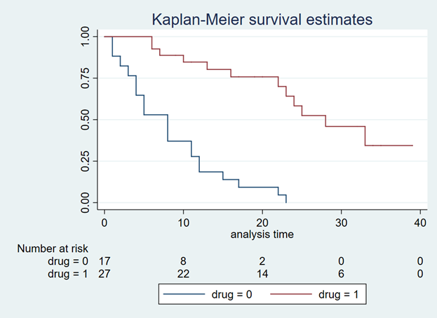
You should go a Kaplan-Meier curve that illustrates the survival probability of 2 dissimilar drugs (Figure ane). The Y-centrality denotes the survival probability and the Ten-axis denotes the fourth dimension in months. Below the effigy is the number at risk for the 2 drug comparators. We will need this to generate our Weibull curves. (If possible, discover a Kaplan-Meier curve with the number at risk. It will make the Weibull curve generation easier.) Alternative methods exist to use Kaplan-Meier curves without the number at risk, but they will non be discussed in this tutorial.

Effigy 1. Kaplan-Meier curve.

Yous will need to download the "Engauge Digitizer" application to convert this Kaplan-Meier curve into a *.CSV file with the appropriate data points. This will help you lot to develop an accurate survival curve based on the Kaplan-Meier curve. You can download the "Engauge Digitizer" application here: https://markummitchell.github.io/engauge-digitizer/

After you download "Engauge Digitizer," open information technology and import the Kaplan-Meier file. Your interface should expect like the following:

Figure 2. Engauge Digitizer interface.

The right console guides y'all in digitizing your Kaplan-Meier figure. Follow this guide carefully. I will non get into how to utilise "Engauge Digitizer;" nevertheless a YouTube video tutorial to utilize Engauge Digitizer was developed by Symmetry Solutions and is available here.

We volition utilise the top Kaplan-Meier bend (which is highlighted with blue crosshairs in Figure 3) to generate our Weibull curves.

Effigy 3. Select the top curve to digitize.

Afterward you digitize the effigy, you will export the data as a *.CSV file. The *.CSV file should accept two columns corresponding to the X- and Y-axes of the Kaplan-Meier figure. Figure 4 has the X values end at row 20 to fit onto the page, but this extends till the cease of the Kaplan-Meier time catamenia, which is forty.

Figure 4. *.CSV file generated from the Kaplan-Meier curve (truncated to fit onto this page).

I usually superimpose the "Engauge Digitizer" results with the actual Kaplan-Meier figure to evidence to myself (and others) that the curves are exactly the same (Figure five). This is a practiced practice to convince yourself that your digitized data properly reflects the Kaplan-Meier curve from the report.

Figure 5. Kaplan-Meier bend superimposed on elevation of the Engauge Digitizer curve.

Now, that nosotros have the digitized version of the Kaplan-Meier, we need to format the information to import into the Weibull curve generator. Hoyle and Henley wrote a paper that explains their methods for using the results from the digitizer to generate Weibull curves.[i] Nosotros volition utilise the Excel template they developed in order to generate the relevant Weibull bend parameters. (The link to the Excel template is provided at the end of this tutorial.)

I always format the data to match the Excel template adult past Hoyle and Henley. The blue box indicates the number at risk at the fourth dimension points denoted past Figure 1 and the blood-red box highlights the evenly spaced time intervals that I estimated (Figure half dozen).

Figure 6. Setting upwardly your data using the template from Hoyle and Henley.

In social club to find the survival probability at each "Showtime fourth dimension" listed in the Excel template by Hoyle and Henley, linear interpolation is used. [You tin can utilise other methods to estimate the survival probability between each time points given the data on Figure 3 (e.g., concluding observation carried forrard); however, I adopt to use linear interpolation.] In Figure vii, the survival probabilities (Y) correspond to a fourth dimension (X) that was generated past the digitizer. At present, we desire to find the Y value respective to the X values on the Excel template.

Figure seven. Generating the Y-values using linear interpolation.

Figure viii illustrates how we apply the linear interpolation to estimate the Y value that corresponds with the X values from the Excel template developed past Hoyle and Henley. For example, if you were interested in finding the Y value at Ten = 10, the you would need to input the following into the linear interpolation equation using the following expression:

This yields a Y value of 0.866993, which is approximately 0.87.

Figure viii. Y values are generated using linear interpolation.

After generating the Y values corresponding to the Start time from Figure 5, yous can enter them into the Excel template past Hoyle and Henley (Effigy nine). Effigy 9 illustrates the inputted survival probabilities into the Excel template.

Figure 9. Survival probabilities are entered after estimating them from linear interpolation.

After the "Empirical survival probability Due south(t)" is populated, you will need to go to the "R Data" worksheet in the Excel template and save this data as a *.CSV file. In this example, I saved the data as "example_data.csv" (Figure 10).

Figure 10. Information is saved as "example_data.csv."

Then I used the following R code to judge the Weibull parameters. This R code is located in the "Curve fitting 'R' code" in the Excel templated developed by Hoyle and Henley. (I modified the R code written by Hoyle and Henley to permit for a *.CSV file import.)

rm(list=ls(all=True))    library(survival)     #    Step 4.   Update directory name and text file proper name in line below    setwd("insert the folder path where the information is stored") information<- read.csv("example_data.csv") attach(data) data      times_start <-c(  rep(start_time_censor, n_censors), rep(start_time_event, n_events) )   times_end <-c(  rep(end_time_censor, n_censors), rep(end_time_event, n_events)  )     #  adding times for patients at risk at last fourth dimension point  ######code does non apply because 0 at chance at last fourth dimension bespeak   ######code does not apply because 0 at take chances at last fourth dimension point    #   Step 5. cull one of these part forms   (WEIBULL was called for the example) model <- survreg(Surv(times_start, times_end, type="interval2")~1, dist="exponential")   # Exponential part, interval censoring  model <- survreg(Surv(times_start, times_end, type="interval2")~i, dist="weibull")   # Weibull function, interval censoring  model <- survreg(Surv(times_start, times_end, blazon="interval2")~i, dist="logistic")   # Logistic function, interval censoring    model <- survreg(Surv(times_start, times_end, type="interval2")~1, dist="lognormal")   # Lognormal function, interval censoring  model <- survreg(Surv(times_start, times_end, type="interval2")~one, dist="loglogistic")   # Loglogistic function, interval censoring   #   Compare AIC values   n_patients <- sum(n_events) +  sum(n_censors)    -ii*summary(model)$loglik[1] + 1*2   #  AIC for exponential distribution  -two*summary(model)$loglik[1] + one*log(n_patients)   #  BIC exponential     -2*summary(model)$loglik[1] + 2*2   #  AIC for 2-parameter distributions     -2*summary(model)$loglik[one] + 2*log(n_patients)   #  BIC for 2-parameter distributions     intercept <- summary(model)$table[1]   # intercept parameter     log_scale <- summary(model)$tabular array[2]   # log scale parameter      #  output for the example of the Weibull distribution    lambda <- i/ (exp(intercept))^ (1/exp(log_scale))    # l for Weibull, where S(t) = exp(-lt^1000)    gamma <- 1/exp(log_scale)     # k for Weibull, where S(t) = exp(-lt^g)   (1/lambda)^(i/gamma) * gamma(1+1/gamma)    # mean time for Weibull distrubtion     #  For the Probabilistic Sensitivity Assay, we need the Cholesky matrix, which captures the variance and covariance of parameters     t(chol(summary(model)$var))    #  Cholesky matrix     #  Simulate variability of mean for Weibull  library(MASS)     simulations <- 10000  # number of simulations for standard deviation of mean     sim_parameters <- mvrnorm(due north=simulations, summary(model)$table[,one],  summary(model)$var  )   # simulates simulations from multivariate normal     intercepts <- sim_parameters[,1]   # intercept parameters    log_scales <- sim_parameters[,2]   # log calibration parameters    lambdas <- ane/ (exp(intercepts))^ (1/exp(log_scales))    # 50 for Weibull, where Southward(t) = exp(-lt^g)     gammas <- 1/exp(log_scales)     # one thousand for Weibull, where Southward(t) = exp(-lt^g)     means <- (one/lambdas)^(1/gammas) * gamma(1+one/gammas)    # mean times for Weibull distrubtion  sd(means)   # standard departure of hateful survival     # consider adding this (from Arman October 2016) to plot KM  km <- survfit(Surv(times_start, times_end, type="interval2")~ one)     summary(km)  plot(km, xmax=600, xlab="Fourth dimension (Days)", ylab="Survival Probability")                  

In that location are several elements generated past the higher up R code that you demand to tape, including the intercept and log-scale:

> intercept [1] 3.494443 > log_scale [1] -0.5436452                  

Once y'all take this, input them into the Excel template sheet titled "Number events & censored," which is the aforementioned sheet you used to generate the survival probabilities after entering the data from the "Engauge Digitizer." Effigy 11 illustrates where these parameters are entered (red square).

Figure eleven. Enter the intercept and log scale parameters into the Excel template developed by Hoyle and Henley.

Yous can cheque the fit of the Weibull curve to the observed Kaplan-Meier curve in the tab "Kaplan-Meier." Figure 12 illustrates the Weibull fit's approximation of the observed Kaplan-Meier curve.

Effigy 12. Weibull fit (cerise curve) of the observed Kaplan-Meier bend (bluish line).

From Figure xi, we also have the lambda (λ=0.002433593) and gamma (γ=1.722273465) parameters which we'll employ to simulate survival using a Markov model.

SUMMARY

In the next blog, nosotros volition discuss how to use the Weibull parameters to generate a survival curve using a Markov model. Additionally, we will acquire how to extrapolate the survival bend beyond the time period used to generate the Weibull parameters for cost-effectiveness studies that use a lifetime horizon.

REFERENCES

Location of Excel spreadsheet developed by Hoyle and Henley (Update 02/17/2019: I learned that Martin Hoyle is not hosting this on his Exeter site due to a contempo change in his academic appointment. For those interested in getting admission to the Excel spreadsheet used in this blog, please download it at this link ).

Location of the Markov model used in this practise is bachelor in the post-obit link:

https://www.dropbox.com/sh/ztbifx3841xzfw9/AAAby7qYLjGn8ZfbduJmAsVva?dl=0

Symmetry Solutions. "Engauge Digitizer—Catechumen Images into Useable Information." Available at the following url: https://www.youtube.com/watch?v=EZTlyXZcRxI

Engauge Digitizer: Marking Mitchell, Baurzhan Muftakhidinov and Tobias Winchen et al, "Engauge Digitizer Software." Webpage: http://markummitchell.github.io/engauge-digitizer [Last Accessed: February 3, 2018].

1. Hoyle MW, Henley W. Improved curve fits to summary survival data: awarding to economical evaluation of wellness technologies. BMC Med Res Methodol 2011;eleven:139.

ACKNOWLEDGMENTS

I desire to thank Solomon J. Lubinga for helping me with my first effort to use Weibull curves in a cost-effectiveness analysis. His deep agreement and patient tutelage are characteristics that I aspire to. I also want to thank Elizabeth D. Brouwer for her comments and edits, which have improved the readability and menstruum of this blog. Additionally, I desire to thank my doctoral dissertation chair, Beth Devine, for her edits and mentorship.

ohearnwourease.blogspot.com

Source: https://mbounthavong.com/blog/2018/3/15/generating-survival-curves-from-study-data-an-application-for-markov-models-part-1-of-2

Share this post